7 Evolution of Convolutional Neural Networks (CNNs)

“Sometimes the simplest ideas have the greatest impact.” - William of Ockham, philosopher

Convolutional Neural Networks (CNNs) showed their potential with Yann LeCun’s 1989 work on learnable convolutional filters using backpropagation and the successful recognition of handwritten digits with LeNet-5 in 1998. In 2012, AlexNet won the ImageNet Large Scale Visual Recognition Challenge (ILSVRC) with a dominant performance, opening the era of deep learning, especially CNNs. However, after AlexNet, attempts to increase network depth encountered difficulties due to vanishing/exploding gradients.

In 2015, Kaiming He and his team at Microsoft proposed ResNet (Residual Network), which solved this problem through the innovative idea of “residual learning”. ResNet successfully trained a 152-layer deep network, which was previously impossible, and set new standards in image recognition. The core element of ResNet, residual connections, has become an essential component in most deep learning architectures.

This chapter examines the background and development process of CNNs, analyzes the key ideas and structures of ResNet in depth, and explores the Inception module and EfficientNet’s core concepts, which are important milestones in the evolution of CNNs. This will provide a broad understanding of modern CNN architectures.

7.1 The Birth of Convolutional Neural Networks

Challenge: How can computers recognize objects within images like humans do?

Researchers’ Concerns: Early computer vision researchers wanted to extract features from images and recognize objects based on those features, rather than treating images as simple collections of pixel values. However, it was unclear which features were important and how to efficiently extract them.

In the early 1960s, David Hubel and Torsten Wiesel conducted experiments on the visual cortex of cats and discovered that certain neurons selectively responded only to specific visual patterns (e.g., vertical lines, horizontal lines, or edges in a particular direction). They won the Nobel Prize in Physiology or Medicine in 1981 for this research, but at the time, no one expected it would lead to revolutionary advancements in artificial intelligence. Hubel and Wiesel’s discovery provides the biological basis for two core concepts of modern CNNs: convolutional layers and pooling layers.

• Simple Cells: Respond to local features such as edges or line segments with specific orientations. This is similar to how CNN convolutional layers use filters (kernels) to extract local features from images.
• Complex Cells: Exhibit translation invariance over the outputs of simple cells, meaning they respond regardless of the position of a pattern within an image. This is similar to how CNN pooling layers reduce feature map sizes while maintaining some location information.

Category	Description
Simple Cells	Respond to local features like edges or lines with specific orientations
Complex Cells	Exhibit translation invariance, responding to patterns regardless of their position

Note: The table above illustrates the characteristics of simple and complex cells discovered by Hubel and Wiesel. In 1980, Kunihiko Fukushima proposed the Neocognitron, which can be considered the prototype of the CNN. The Neocognitron was composed of multiple layers of S-cells (simple cells) and C-cells (complex cells), allowing it to extract hierarchical features from images and perform pattern recognition that is robust to position changes.

However, at the time, the Neocognitron did not have a established learning algorithm, so filters (weights) had to be set manually. In 1989, Yann LeCun applied the backpropagation algorithm to convolutional neural networks, allowing filters to be learned automatically from data. This gave birth to the modern CNN, which showed excellent performance in handwritten digit recognition under the name LeNet-5.

In 2012, AlexNet won the ImageNet challenge with overwhelming performance, opening the era of deep learning and CNNs. AlexNet had a much deeper and more complex structure than LeNet-5 and was able to efficiently learn large datasets (ImageNet) using parallel computing with GPUs.

7.1.1 Advancements in Digital Signal Processing and Background of CNNs

To deeply understand computer vision and CNNs, it is necessary to examine the development process of digital signal processing (DSP). In 1807, Joseph Fourier proposed the Fourier transform, which states that any periodic function can be decomposed into a sum of sine and cosine functions. This became the foundation of signal processing and enabled the analysis of time-domain signals in the frequency domain.

In particular, with the development of digital computers in the 1960s, the fast Fourier transform (FFT) algorithm was developed, and digital signal processing entered a new era. The FFT allowed for much faster calculation of Fourier transforms, and signal processing technology began to be widely used in various fields such as images, voice, and communication.

In image processing, convolution operations play a core role. Convolution is a basic operation that applies filters (kernels) to input signals (images) to extract desired features or remove noise. Digital filter theory, which developed from the 1960s, enabled various processing such as edge detection, blurring, and sharpening of images. In the late 1960s, the Kalman filter emerged, providing a powerful tool for estimating system states from noisy measurements. The Kalman filter uses a recursive algorithm based on Bayes’ theorem and is essential in computer vision today, including object tracking and robot vision.

These traditional digital signal processing technologies became the theoretical foundation of CNNs. However, existing filters had to be designed manually and had fixed forms, limiting their ability to recognize various patterns. CNNs overcame these limitations by automatically learning optimal filters from data, bringing about a revolution in image recognition.

7.1.2 Digital Filters and Convolution

To understand CNNs, it is first necessary to understand the concept of digital filters. Digital filters are used for two main purposes in signal processing. 1. Signal Separation: Separates the desired signal component from a mixed signal. (For example, when a fetal heartbeat and a mother’s heartbeat are mixed, only the fetal heartbeat is separated) 2. Signal Restoration: Restores distorted or damaged signals to be closer to the original signal. (For example, noise removal from an image, restoration of a blurred image)

One of the most basic digital filters is the Sobel filter. The Sobel filter is a 3x3 matrix used to detect the edge of an image.

!pip install dldna[colab] # in Colab
# !pip install dldna[all] # in your local

%load_ext autoreload
%autoreload 2

import numpy as np
# Sobel filter for vertical edge detection
sobel_vertical = np.array([
    [-1, 0, 1],
    [-2, 0, 2],
    [-1, 0, 1]
])

# Sobel filter for horizontal edge detection
sobel_horizontal = np.array([
    [-1, -2, -1],
    [ 0,  0,  0],
    [ 1,  2,  1]
])

Let’s take a look at what classical digital filters do. The entire code is in chapter_06/filter_utils.py.

import matplotlib.pyplot as plt
from dldna.chapter_07.filter_utils import show_filter_effects, create_convolution_animation
%matplotlib inline

# 테스트용 이미지 URL
IMAGE_URL = "https://raw.githubusercontent.com/opencv/opencv/master/samples/data/building.jpg"

# 필터 효과 시각화
show_filter_effects(IMAGE_URL)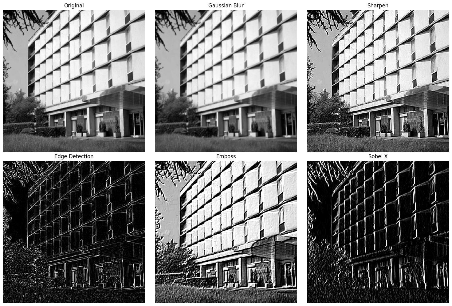

The above example used the following filter:

filters = {
    'Gaussian Blur': cv2.getGaussianKernel(3, 1) @ cv2.getGaussianKernel(3, 1).T,
    'Sharpen': np.array([
        [0, -1, 0],
        [-1, 5, -1],
        [0, -1, 0]
    ]),
    'Edge Detection': np.array([
        [-1, -1, -1],
        [-1, 8, -1],
        [-1, -1, -1]
    ]),
    'Emboss': np.array([
        [-2, -1, 0],
        [-1, 1, 1],
        [0, 1, 2]
    ]),
    'Sobel X': np.array([
        [-1, 0, 1],
        [-2, 0, 2],
        [-1, 0, 1]
    ])
}

This is how these filters work, which is convolution. The filter slides over the image, calculating the sum of element-wise multiplication of the filter and the image portion at each position. This can be expressed by the following equation:

\((I * K)(x, y) = \sum_{i=-a}^{a}\sum_{j=-b}^{b} I(x+i, y+j)K(i, j)\)

Here, \(I\) is the input image and \(K\) is the kernel (filter). \((x,y)\) are the coordinates of the output pixel, \((i,j)\) are the coordinates inside the kernel, and \(a\) and \(b\) are the half sizes of the kernel horizontally and vertically.

Convolution operations are easier to understand visually. The animation below shows the process of convolution operation.

from dldna.chapter_07.conv_visual import create_conv_animation
from IPython.display import HTML
%matplotlib inline

# 애니메이션 생성 및 표시
animation = create_conv_animation()

# js_html = animation.to_jshtml()
# display(HTML(f'<div style="width:700px">{js_html}</div>'))

# html_video = animation.to_html5_video()
# display(HTML(f'<div style="width:700px">{html_video}</div>'))

display(animation)

Once Loop Reflect

The biggest limitation of digital filters is their fixed characteristics. Traditional filters such as Sobel and Gaussian are manually designed to detect specific patterns only, so they have limitations in recognizing complex and diverse patterns. They are also vulnerable to changes in image size or rotation and cannot automatically learn multiple layers of features. These limitations led to the development of data-driven learnable filters like CNNs.

7.1.2 Characteristics and Structure of CNN

CNN efficiently learns the spatial hierarchy in images by mimicking biological visual processing mechanisms.

Learnable Filters

The biggest characteristic of CNN is that it uses filters learned automatically from data instead of manually designed filters (e.g., Sobel, Gabor filters). This allows CNN to learn feature extractors optimized for specific tasks (e.g., image classification, object detection) on its own.

import torch
import torch.nn as nn
import torch.nn.functional as F

class SimpleCNN(nn.Module):
    def __init__(self):
        super().__init__()
        # Multiple learnable filters: 32 (channels) of 3x3 filter weight matrices + 32 biases
        self.conv1 = nn.Conv2d(1, 32, kernel_size=3, padding=1)
        # Multiple learnable filters: For 32 input channels, 64 output channels of 3x3 filter weight matrices + 64 biases
        self.conv2 = nn.Conv2d(32, 64, kernel_size=3, padding=1)

    def forward(self, x):
        x = F.relu(self.conv1(x))
        x = F.relu(self.conv2(x))
        return x

In the SimpleCNN example above, conv1 and conv2 are convolutional layers with learnable filters. The first argument of nn.Conv2d is the number of input channels, the second argument is the number of output channels (the number of filters), kernel_size is the size of the filter, and padding plays a role in adjusting the size of the output feature map by filling 0 around the input image.

Hierarchical Feature Extraction

CNN extracts hierarchical features of an image through multiple layers of convolution and pooling operations.

• Low-level features: Detect basic visual features (low-level features) such as edges, lines, and color changes.
• Mid-level features: Learn mid-level features such as texture, pattern, and simple shapes.
• High-level features: Recognize abstract and high-level features such as parts of objects and the overall structure of objects.

This hierarchical feature extraction is similar to the way the human visual system processes visual information step by step.

import torch
import torch.nn as nn
import torch.nn.functional as F

class HierarchicalCNN(nn.Module):
    def __init__(self):
        super().__init__()
        # Low-level feature extraction
        self.conv1 = nn.Conv2d(3, 64, 3, padding=1)
        self.bn1 = nn.BatchNorm2d(64)

        # Mid-level feature extraction
        self.conv2 = nn.Conv2d(64, 128, 3, padding=1)
        self.bn2 = nn.BatchNorm2d(128)

        # High-level feature extraction
        self.conv3 = nn.Conv2d(128, 256, 3, padding=1)
        self.bn3 = nn.BatchNorm2d(256)

    def forward(self, x):
        # Low-level features (edges, textures)
        x = F.relu(self.bn1(self.conv1(x)))

        # Mid-level features (patterns, partial shapes)
        x = F.relu(self.bn2(self.conv2(x)))

        # High-level features (object parts, overall structure)
        x = F.relu(self.bn3(self.conv3(x)))
        return x

The example of HierarchicalCNN above shows a CNN that uses three convolutional layers to extract low-level, middle-level, and high-level features. In reality, many more layers are stacked to learn even more complex features.

Spatial Hierarchy and Pooling

Each layer of the CNN typically consists of convolution operations, activation functions (such as ReLU), and pooling operations.

• Convolutional Layer: Extracts features from the input feature map using filters.
• Activation Function: Applies a non-linear function such as ReLU to add non-linearity to the network.
• Pooling Layer: Reduces the size of the feature map (downsampling) to decrease the amount of computation and enhance translation invariance, i.e., enabling the network to recognize the same object even if it is slightly moved within the image. Typically, max pooling is used.

Thanks to these structural characteristics, CNNs can effectively learn spatial information from images and extract robust features that are resistant to changes in the location of objects within the image.

Parameter Sharing

Parameter sharing is a key efficiency mechanism of CNNs. The same filter is used at all locations of the input image (or feature map). This is based on the assumption that the same features are detected at each location. (For example, a vertical line filter detects vertical lines regardless of whether it’s in the top-left or bottom-right of the image.)

1. Memory Efficiency: Since the parameters of the filters are shared across all locations, the number of parameters in the model is drastically reduced. For instance, suppose we have a convolutional layer with 64 filters of size 3x3 applied to a 32x32 color (3-channel) image. Each filter has 3x3x3 = 27 parameters. Without parameter sharing, we would need a different filter for each of the 32x32 locations, resulting in (32x32) x (3x3x3) x 64 parameters. However, with parameter sharing, we only need 27 x 64 + 64 (bias) = 1792 parameters.

2. Statistical Efficiency: Since the same filter learns features from multiple locations of the image, we can learn effective feature extractors with a smaller number of parameters. This improves the generalization performance of the model.

3. Parallelization: Convolution operations are highly parallelizable since each filter is applied independently and then combined.

from dldna.chapter_07.param_share import compare_parameter_counts, show_example

# 다양한 입력 크기에 따른 비교. CNN 입출력 채널을 1로 고정.
input_sizes = [8, 16, 32, 64, 128]
comparison = compare_parameter_counts(input_sizes)
print("\nParameter Count Comparison:")
print(comparison)

# 32x32 입력에 대한 상세 예시
show_example(32)

Parameter Count Comparison:
  Input Size  Conv Params  FC Params  Ratio (FC/Conv)
0        8x8           10       4160            416.0
1      16x16           10      65792           6579.2
2      32x32           10    1049600         104960.0
3      64x64           10   16781312        1678131.2
4    128x128           10  268451840       26845184.0

Example with 32x32 input:
CNN parameters: 10 (fixed)
FC parameters: 1,049,600
Parameter reduction: 99.9990%

Receptive Field

The receptive field refers to the size of the input image area that affects the output of a particular neuron. In CNNs, as the convolutional and pooling layers progress, the receptive field gradually increases.

• Early layers: Have small receptive fields, so they detect local features (e.g., edges, points).
• Deeper layers: Have larger receptive fields, so they learn more abstract features (e.g., parts of objects, entire objects) by considering a wider context.

Thanks to this hierarchical feature extraction and the expanding receptive field, CNNs can achieve excellent performance in image recognition.

In conclusion, CNNs, inspired by biological visual processing systems, have led to innovative advances in image recognition and computer vision through their core features, including convolutional operations, pooling operations, learnable filters, parameter sharing, and hierarchical feature extraction.

7.1.3 Mathematical Expression and Implementation of CNN

The mathematical expression of CNN is as follows:

\((F * K)(p) = \sum_{s+t=p} F(s)K(t) = \sum_{i}\sum_{j} F(i,j)K(p_x-i, p_y-j)\)

Here, \(F\) represents the input feature map, and \(K\) represents the kernel. In actual implementation, considering multiple channels and batch processing, it is extended as follows:

\(Y_{n,c_{out},h,w} = \sum_{c_{in}}\sum_{i=0}^{k_h-1}\sum_{j=0}^{k_w-1} X_{n,c_{in},h+i,w+j} \cdot W_{c_{out},c_{in},i,j} + b_{c_{out}}\)

Here: - \(n\) is the batch index - \(c_{in}\), \(c_{out}\) are input/output channels - \(h\), \(w\) are height and width - \(k_h\), \(k_w\) are kernel sizes - \(W\) is the weight, \(b\) is the bias

A class that implements 2D convolution and max pooling for learning purposes, referencing PyTorch source code, is in chapter_06/simple_conv.py. For educational purposes, CUDA optimization is not used, and exception handling is removed, using a for loop instead. Since detailed comments are included in the source code, description of the class will be omitted.

import torch
import matplotlib.pyplot as plt
from dldna.chapter_07.simple_conv import SimpleConv2d, SimpleMaxPool2d
# %matplotlib inline  # This line is only needed in Jupyter/IPython environments

# Input data creation (e.g., 1 image, 1 channel, 6x6 size)
x = torch.tensor([
    [1, 2, 3, 4, 5, 6],
    [7, 8, 9, 10, 11, 12],
    [13, 14, 15, 16, 17, 18],
    [19, 20, 21, 22, 23, 24],
    [25, 26, 27, 28, 29, 30],
    [31, 32, 33, 34, 35, 36]
], dtype=torch.float32).reshape(1, 1, 6, 6)

# SimpleConv2d test
conv = SimpleConv2d(in_channels=1, out_channels=2, kernel_size=3, padding=1)
conv_output = conv(x)

# SimpleMaxPool2d test
pool = SimpleMaxPool2d(kernel_size=2)
pool_output = pool(x)

# Visualize results
fig, axes = plt.subplots(1, 3, figsize=(15, 5))

# Original image
axes[0].imshow(x[0, 0].detach().numpy(), cmap='viridis')
axes[0].set_title('Original Image')

# Convolution result (first channel)
axes[1].imshow(conv_output[0, 0].detach().numpy(), cmap='viridis')
axes[1].set_title('Conv2d Output (Channel 0)')

# Pooling result
axes[2].imshow(pool_output[0, 0].detach().numpy(), cmap='viridis')
axes[2].set_title('MaxPool2d Output')

for ax in axes:
    ax.axis('off')
plt.tight_layout()
plt.show()

# Print output sizes
print("Input size:", x.shape)
print("Convolution output size:", conv_output.shape)
print("Pooling output size:", pool_output.shape)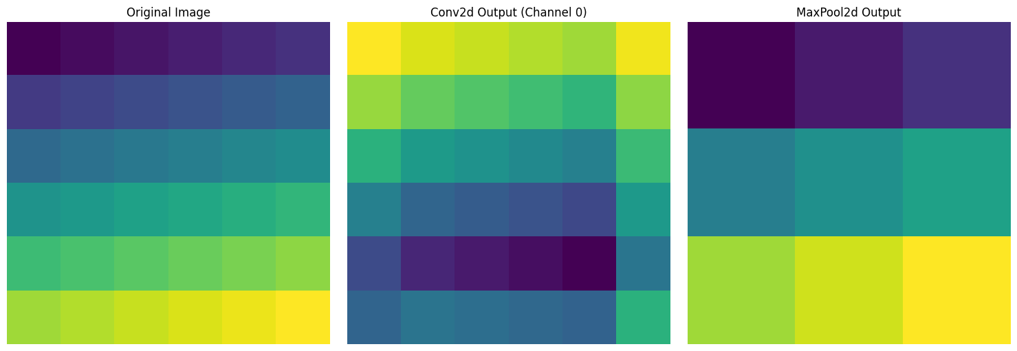

Input size: torch.Size([1, 1, 6, 6])
Convolution output size: torch.Size([1, 2, 6, 6])
Pooling output size: torch.Size([1, 1, 3, 3])

For a 6x6 input image, three results are visualized. The left is the original image with values sequentially increasing from 1 to 36, the center is the result of applying a 3x3 convolution filter, and the right shows the result of applying 2x2 max pooling, reducing the size by half.

Click to view contents (Deep Dive: Frequency Domain Interpretation of Convolutional Operations and the Meaning of 1x1 Convolutions)

Interpretation of Convolution Operation in Frequency Domain and Meaning of 1x1 Convolution

We delve into the interpretation of convolution, a core operation in CNNs, in the frequency domain, and explore the meaning of 1x1 convolution in depth. Through Fourier transform and convolution theorem, we will uncover the hidden meaning behind the convolution operation.

1. Review of Convolution Operation

We briefly review the convolution operation discussed in sections 7.1.2 and 7.1.3. The convolution operation \(I * K\) between a 2D image \(I\) and a kernel (filter) \(K\) is defined as follows:

\((I * K)[i, j] = \sum_{m} \sum_{n} I[i-m, j-n] K[m, n]\)

where \(i\), \(j\) are the pixel positions of the output image, and \(m\), \(n\) are the pixel positions of the kernel. Discrete convolution is a process of sliding the kernel over the image, performing element-wise multiplication and summation in the overlapping regions.

2. Introduction to Fourier Transform

The Fourier transform is a powerful tool for converting signals from the spatial domain to the frequency domain.

• Spatial Domain vs. Frequency Domain: The spatial domain refers to the form of a signal that we typically perceive (e.g., changes in pixel values of an image over time). The frequency domain represents the signal as a composition of various frequency components (e.g., different spatial frequency components contained in an image).

• Definition of Fourier Transform: The Fourier transform decomposes a signal into a sum of sine and cosine functions with different frequencies and amplitudes. For a continuous function \(f(t)\), its Fourier transform \(\mathcal{F}\{f(t)\} = F(\omega)\) is defined as:

  \(F(\omega) = \int_{-\infty}^{\infty} f(t) e^{-j\omega t} dt\)

  where \(j\) is the imaginary unit and \(\omega\) is the angular frequency. The inverse Fourier transform restores the signal from the frequency domain back to the spatial domain.

  \(f(t) = \frac{1}{2\pi} \int_{-\infty}^{\infty} F(\omega) e^{j\omega t} d\omega\)

• Discrete Fourier Transform (DFT) & Fast Fourier Transform (FFT): Since computers cannot handle continuous signals, we use the discrete Fourier transform (DFT). DFT applies the Fourier transform to discrete data. The fast Fourier transform (FFT) is an efficient algorithm for computing DFT. The formula for DFT is:

  \(X[k] = \sum_{n=0}^{N-1} x[n] e^{-j(2\pi/N)kn}\), \(k = 0, 1, ..., N-1\)

  where \(x[n]\) is the discrete signal, \(X[k]\) is the result of DFT, and \(N\) is the length of the signal.

3. Convolution Theorem

The convolution theorem describes an important relationship between the convolution operation and the Fourier transform. The key point is that convolution in the spatial domain becomes a simple multiplication in the frequency domain.

• Convolution Theorem: The Fourier transform of the convolution \(f(t) * g(t)\) of two functions \(f(t)\) and \(g(t)\) is equal to the product of their individual Fourier transforms.

  \(\mathcal{F}\{f * g\} = \mathcal{F}\{f\} \cdot \mathcal{F}\{g\}\)

  That is, if \(F(\omega)\) and \(G(\omega)\) are the Fourier transforms of \(f(t)\) and \(g(t)\) respectively, then the Fourier transform of \(f(t) * g(t)\) is \(F(\omega)G(\omega)\).

• Interpretation in the frequency domain: The convolution theorem allows us to interpret the convolution operation in the frequency domain. The convolution filter plays a role in emphasizing or suppressing specific frequency components of the input signal. Multiplication in the frequency domain is equivalent to adjusting the amplitude of the corresponding frequency components.

4. Frequency Response of Convolution Filters

Analyzing the frequency response of various convolution filters reveals which frequency components are passed through and which are blocked.

• Visualizing frequency response: The frequency response can be obtained by calculating the Fourier transform of the filter. The frequency response is typically represented in terms of magnitude and phase. The magnitude represents the change in amplitude of each frequency component, while the phase represents the phase shift.

• Filter types:

  • Low-pass filter: Passes low-frequency components and blocks high-frequency components. It has a blurring effect on images (e.g., Gaussian filter).
  • High-pass filter: Passes high-frequency components and blocks low-frequency components. It has an edge-enhancing effect on images (e.g., Sobel filter).
  • Band-pass filter: Only passes a specific frequency band and blocks the rest.

The following is an example of visualizing the frequency response of Sobel and Gaussian filters. (Running the code generates an image.)

import numpy as np
import matplotlib.pyplot as plt
from scipy.signal import convolve2d

def plot_frequency_response(kernel, title):
    # Calculate the 2D FFT of the kernel
    kernel_fft = np.fft.fft2(kernel, s=(256, 256)) # Zero-padding for better visualization
    kernel_fft_shifted = np.fft.fftshift(kernel_fft) # Shift zero frequency to center

    # Calculate the magnitude and phase
    magnitude = np.abs(kernel_fft_shifted)
    phase = np.angle(kernel_fft_shifted)

    # Plot the magnitude response
    plt.figure(figsize=(12, 6))
    plt.subplot(1, 2, 1)
    plt.imshow(np.log(1 + magnitude), cmap='gray') # Log scale for better visualization
    plt.title(f'{title} - Magnitude Response')
    plt.colorbar()
    plt.axis('off')


    #Plot the phase response
    plt.subplot(1, 2, 2)
    plt.imshow(phase, cmap='hsv')
    plt.title(f'{title} - Phase Response')
    plt.colorbar()
    plt.axis('off')
    plt.show()

Example kernels

sobel_x = np.array([[-1, 0, 1], [-2, 0, 2], [-1, 0, 1]]) sobel_y = np.array([[-1, -2, -1], [0, 0, 0], [1, 2, 1]]) gaussian = np.array([[1, 4, 6, 4, 1], [4, 16, 24, 16, 4], [6, 24, 36, 24, 6], [4, 16, 24, 16, 4], [1, 4, 6, 4, 1]]) / 256.0

Plot frequency responses

plot_frequency_response(sobel_x, ‘Sobel X Filter’) plot_frequency_response(sobel_y, ‘Sobel Y Filter’) plot_frequency_response(gaussian, ‘Gaussian Filter’)

5. Interpretation of 1x1 Convolution in the Frequency Domain

1x1 convolution performs operations between channels while maintaining spatial information.

• Linear Combination of Channels: 1x1 convolution performs a linear combination of channels at each pixel location. This can be interpreted as a weighted sum of the frequency components of each channel in the frequency domain. Therefore, the weights of the 1x1 convolution filter represent the importance of each channel’s frequency component.

• Adjusting Correlations and Reconstructing Features: 1x1 convolution adjusts the correlations between channels. It combines channels with strong correlations or removes unnecessary channels to reconstruct feature representations.

• Role in Inception Modules: In Inception modules, 1x1 convolution plays two important roles.

  • Dimensionality Reduction: Reduces the number of channels, decreasing computational costs.
  • Adding Non-Linearity: Applies non-linear activation functions like ReLU after 1x1 convolution to increase the model’s expressiveness. From a frequency response perspective, it allows mixing channels with different frequency responses to create more complex frequency responses.

7.1.4 Calculating Learnable Parameters of CNN

Calculating the number of learnable parameters in a CNN is crucial for network design and optimization. Let’s break it down step by step.

1. Basic Convolution Layer

conv = nn.Conv2d(in_channels=1, out_channels=32, kernel_size=3)

The parameter calculation is as follows: - Each filter size: 3 × 3 × 1 (kernel size² × input channel) - Number of filters: 32 (output channel) - Bias: 32 (same as output channel) - Total parameters = (3 × 3 × 1) × 32 + 32 = 320

2. Max Pooling Layer

maxpool = nn.MaxPool2d(kernel_size=2, stride=2)

• No learnable parameters
• Simply performs an operation to select the maximum value in a 2×2 area
• Only reduces the size of the feature map (height and width are both 1/2)

3. Convolution with Padding

conv = nn.Conv2d(in_channels=3, out_channels=64, kernel_size=3, padding=1)

Padding only affects the output size, not the number of parameters. - Each filter size: 3 × 3 × 3 - Number of filters: 64 - Total parameters = (3 × 3 × 3) × 64 + 64 = 1,792

4. Combination of Convolution and Pooling with Stride

conv = nn.Conv2d(in_channels=64, out_channels=128, kernel_size=3, stride=2)
maxpool = nn.MaxPool2d(kernel_size=2, stride=2)

• Convolution parameters = (3 × 3 × 64) × 128 + 128 = 73,856
• Pooling parameters = 0
• Total parameters = 73,856

Output size calculation:

Convolution output size = ((input size + 2×padding - kernel size) / stride) + 1
Pooling output size = ((input size - pooling size) / pooling stride) + 1

5. Example of Complex Structure (Basic Block of ResNet)

class BasicBlock(nn.Module):
    def __init__(self, in_channels=64, out_channels=64):
        self.conv1 = nn.Conv2d(in_channels, out_channels, kernel_size=3, padding=1)
        self.bn1 = nn.BatchNorm2d(out_channels)
        self.conv2 = nn.Conv2d(out_channels, out_channels, kernel_size=3, padding=1)
        self.bn2 = nn.BatchNorm2d(out_channels)
        self.maxpool = nn.MaxPool2d(kernel_size=2, stride=2)

Parameter calculation. 1. First convolution: (3 × 3 × 64) × 64 + 64 = 36,928 2. First batch normalization: 64 × 2 = 128 (gamma and beta) 3. Second convolution: (3 × 3 × 64) × 64 + 64 = 36,928 4. Second batch normalization: 64 × 2 = 128 5. Max pooling: 0

Total parameters = 74,112

This parameter count calculation is crucial for understanding the model’s complexity, predicting memory requirements, and evaluating the risk of overfitting. In particular, the pooling layer effectively reduces the size of the feature map without parameters, making a significant contribution to improving computational efficiency.

7.1.5 CNN: Feature Extraction and Abstraction Learning

The core of CNNs lies in extracting image features through “learnable filters” and combining them hierarchically to learn more abstract representations. This process starts with the concrete details of an image and progresses to understanding abstract meanings (e.g., object categories), which can be divided into two main aspects.

1. Feature Extraction and Transformation: Extract features from local regions of an image and leave only meaningful features through nonlinear activation functions.
2. Increasing Filters and Expanding Abstract Space: As the layers deepen, increase the number of filters (channels) to learn more diverse and abstract features.

1. Feature Extraction and Transformation

The convolutional layers of CNNs apply learnable filters to the input image (or feature maps from previous layers) to extract features. Each filter is learned to respond to specific patterns in the image (e.g., edges, textures, shapes). This process involves the following steps.

• Convolution Operation: The filter interacts with local regions of the image (receptive field) and outputs a value indicating whether the specific pattern exists in that region. Through this process, a feature map is generated at each position of the image, showing the strength of the pattern detected by the filter.
• Activation Function: The result of the convolution operation (feature map) passes through a nonlinear activation function like ReLU. The activation function only allows features with values above a certain threshold to pass through to the next layer, ignoring others. This helps the network focus on important features and eliminate unnecessary information, leading to sparse representation.
• Pooling (Optional): Pooling layers reduce the size of feature maps (downsampling) while enhancing translation invariance. For example, max pooling retains only the feature with the highest value within a specific region (e.g., 2x2) and discards the rest.

Through these processes, each convolutional layer of a CNN transforms the input image into a feature space. This feature space is more abstract than the original pixel space and contains more useful information for tasks like classification or object detection.

2. Increasing Filters and Expanding Abstract Space

CNNs have a deep structure composed of multiple layers of convolution and pooling operations. As you progress through each layer, the spatial dimensions (width, height) of feature maps generally decrease, while the number of filters (channels) increases. This is the core mechanism by which CNNs learn abstraction.

• Spatial Dimension Reduction: Convolution operations with a stride greater than 1 or pooling reduce the spatial dimensions of feature maps. This decreases computational complexity and enhances translation invariance, allowing objects to be recognized even if they are slightly moved within an image.
• Channel Increase: Each convolutional layer uses multiple filters to capture various aspects of the input feature map.
  • Early Layers: Detect low-level features such as edges, color changes. These low-level features represent basic components of the image.
  • Middle Layers: Combine low-level features from early layers to detect mid-level features like textures, patterns, and simple shapes.
  • Deep Layers: Combine features from previous layers to detect high-level, abstract features such as parts of objects (eyes, nose, mouth), and further, the objects themselves (people, cars, animals). An increase in the number of filters (channels) means that the dimension of features used by CNN to represent an image increases. In the early layers, it focuses on the specific details of the image, while in the deeper layers, it learns the information necessary to grasp the abstract meaning of the image. This is similar to the process by which humans look at objects, first paying attention to detailed parts and then gradually grasping the overall shape and meaning.

A Representative Example of CNN Layer Structure (VGGNet):

The following is a figure showing the VGGNet architecture. VGGNet is a representative model that systematically studied the effect of CNN depth on performance.

• VGGNet Architecture:

VGG16 architecture.
Source: K. Simonyan, A. Zisserman, “Very deep convolutional networks for large-scale image recognition,” arXiv:1409.1556, 2014.

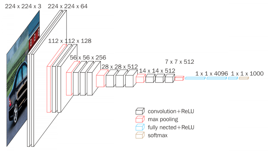
As can be seen in the figure, VGGNet has a structure in which several convolutional layers and pooling layers are stacked. As each layer passes through, the spatial size of the feature map decreases, and the number of channels increases. This visually shows the process by which CNN transforms an image from a low-dimensional specific representation (pixel values) to a high-dimensional abstract representation (object type).

In conclusion, the “learnable filters” of CNN are powerful tools that extract image features and learn more abstract representations by hierarchically combining them. CNN transforms an image into a smaller, deeper, and more abstract representation through multiple layers of convolution and pooling operations, learning key information necessary to grasp the meaning of the image from the data during this process. This feature extraction and abstraction ability is the core reason why CNNs perform excellently in various computer vision tasks such as image recognition, object detection, and image segmentation.

Click to view contents (Deep Dive: Various meanings of the term ‘kernel’ in deep learning and machine learning)

Various Meanings of the Term “Kernel” in Deep Learning and Machine Learning

“Words do not have meaning in themselves, but in the context in which they are used.” - (Basic principle of semantics/pragmatics)

When studying deep learning, machine learning, and signal processing, you often come across the term “kernel”. Since “kernel” can have completely different meanings depending on the context, it can be confusing for those who encounter it for the first time. In this deep dive, we will clarify the various contexts in which “kernel” is used and its meanings, and examine the connections between each usage.

1. Kernel (Convolution Kernel) in Convolutional Neural Networks (CNN)

In CNNs, a kernel is synonymous with a filter. It is a small matrix that performs a convolution operation on the input data (image or feature map) in a convolutional layer.

• Role: Extracts features from local regions (receptive fields) of an image.

• Operation: The kernel moves over the input data, multiplying the values of overlapping pixels with its weights and summing them up (convolution operation). This process outputs a value representing how strongly the pattern (e.g., edge, texture) that the kernel is trying to detect appears at that location.

• Learnable: In CNNs, the weights of the kernel are learned from data through the backpropagation algorithm. In other words, the CNN adjusts the kernel to extract the most useful features for solving a given problem (e.g., image classification).

• Example: Sobel Kernel

  $

  \[\begin{bmatrix} 1 & 0 & -1 \\ 2 & 0 & -2 \\ 1 & 0 & -1 \end{bmatrix}\]

  $ This 3x3 Sobel kernel is used to detect vertical edges in an image.

• Key point: The kernel in a CNN has learnable parameters and plays a role in extracting local features from an image.

2. Kernel (Kernel Function, Kernel Trick) in Support Vector Machines (SVM)

In SVMs, a kernel is a function that calculates the similarity between two data points. SVM maps data to a high-dimensional feature space to solve non-linear classification problems. The kernel trick is a technique that implicitly calculates the inner product in this high-dimensional space without explicitly computing the mapping.

• Role: Maps data to a high-dimensional feature space, transforming non-linear classification problems into linear ones.
• Key point: Efficiently calculates the inner product in the high-dimensional feature space (without explicit mapping).
• Mathematical expression: \(K(\mathbf{x}, \mathbf{y}) = \phi(\mathbf{x}) \cdot \phi(\mathbf{y})\)
  • \(K(\mathbf{x}, \mathbf{y})\): Kernel function (similarity between two input vectors \(\mathbf{x}\) and \(\mathbf{y}\))
  • \(\phi(\mathbf{x})\): Function that maps the input vector \(\mathbf{x}\) to the high-dimensional feature space
  • \(\cdot\): Inner product
• Notable kernel functions:
  • Linear Kernel: \(K(\mathbf{x}, \mathbf{y}) = \mathbf{x}^T \mathbf{y}\) (simple dot product)
  • Polynomial Kernel: \(K(\mathbf{x}, \mathbf{y}) = (\gamma \mathbf{x}^T \mathbf{y} + r)^d\)
  • RBF Kernel (Radial Basis Function Kernel, Gaussian Kernel): \(K(\mathbf{x}, \mathbf{y}) = \exp(-\gamma \|\mathbf{x} - \mathbf{y}\|^2)\) (most widely used)
  • Sigmoid Kernel: \(K(\mathbf{x}, \mathbf{y}) = \tanh(\gamma \mathbf{x}^T \mathbf{y} + r)\)
• Core: The kernel in SVM is a function that measures the similarity between data and solves nonlinear problems through an implicit mapping to high-dimensional feature space.

3. Kernels in Probability and Statistics (Kernel Density Estimation)

In probability and statistics, a kernel is a non-negative function used in kernel density estimation (KDE) that is symmetric around the origin and has an integral value of 1. KDE is a non-parametric method for estimating the probability density function based on given data (samples).

• Role: A “weight function” used to estimate the density around data points.
• Core: By “overlaying” the kernel function over each data point, the overall distribution of the data is smoothly expressed.
• Mathematical Expression: \(\hat{f}(x) = \frac{1}{nh} \sum_{i=1}^{n} K\left(\frac{x - x_i}{h}\right)\)
  • \(\hat{f}(x)\): The estimated probability density at \(x\)
  • \(n\): The number of data points
  • \(h\): Bandwidth - a parameter that controls the “width” of the kernel (smoothing parameter)
  • \(K(\cdot)\): The kernel function
  • \(x_i\): The \(i\)th data point
• Notable kernel functions:
  • Gaussian Kernel: \(K(x) = \frac{1}{\sqrt{2\pi}} e^{-\frac{1}{2}x^2}\) (most widely used)
  • Epanechnikov Kernel: \(K(x) = \frac{3}{4}(1 - x^2) \text{ if } |x| \le 1\)
  • Uniform Kernel (Box Kernel): \(K(x) = \frac{1}{2} \text{ if } |x| \le 1\)
• Core: The kernel in KDE serves as a weight function for estimating the probability density function.

4. Operating System Kernels

In computer science, particularly in the field of operating systems, a kernel is the core component of an operating system. It acts as an interface between hardware and applications and operates at the lowest level of the system.

• Roles:
  • Process management
  • Memory management
  • File system management
  • Input/output (I/O) management
  • Hardware resource management
• Examples: Linux kernel, Windows NT kernel, macOS’s XNU kernel

Summary and Comparison

Field	Meaning of Kernel	Core Role
CNN	Filter performing convolutional operation (learnable weight matrix)	Extracting local features of an image
SVM	Function calculating similarity between two data points (implicit mapping to high-dimensional feature space)	Mapping nonlinear data to high-dimensional space to make it linearly separable
Probabilistic/Statistical (KDE)	Weight function for estimating probability density function	Smoothing estimation of data distribution
Operating System	Core component of operating system (interface between hardware and application)	Managing system resources, hardware abstraction
Linear Algebra	Null space of linear transformation (or matrix), i.e., set of vectors \(\mathbf{x}\) satisfying \(A\mathbf{x}=\mathbf{0}\) (for linear mapping \(T:V→W\), $(T)={∈V∣T()=} $)	Representing characteristics of linear transformation

In deep learning, especially in CNN, “kernel” usually refers to a convolution filter. However, when encountering other machine learning algorithms such as SVM or Gaussian process, it should be noted that it can also mean kernel function. It is crucial to accurately understand the meaning of “kernel” according to the context.

7.2 The Emergence of ResNet

Challenge: How to effectively deepen the neural network while stably training without gradient vanishing/exploding problems?

Researcher’s Dilemma: As CNNs showed excellent performance in image recognition, researchers wanted to create deeper networks. However, as the network deepened, the problem of gradients disappearing (vanishing gradients) or exploding (exploding gradients) during backpropagation occurred, and learning was not properly conducted. The simple repetition of linear transformations limited the expressive power of deep networks. How can we overcome this fundamental limitation and maximize the depth of neural networks?

When CNNs achieved remarkable success in image recognition, researchers naturally asked, “Can’t a deeper network achieve better performance?” In theory, a deeper network should be able to learn more complex and abstract features. However, in reality, as the network deepened, the phenomenon of training error increasing occurred.

7.2.1 The Problem of Deep Neural Networks and the Birth of ResNet

In 2015, a Microsoft research team (Kaiming He et al.) published a paper presenting a groundbreaking solution to this problem. They experimentally revealed that the difficulty of deep neural network learning is not due to overfitting, but rather the difficulty of optimization that cannot even reduce the error for the training data.

The research team observed that a 56-layer neural network had a larger error on the training data than a 20-layer neural network. This was a result that contradicted intuition, which suggested that a 56-layer network should be able to perform at least as well as a 20-layer network (since the 56-layer network can express the function of the 20-layer network by learning an identity mapping with the remaining 36 layers). Thus, they posed the fundamental question: “Why can’t neural networks learn even a simple identity mapping as they deepen?”

To solve this problem, the research team proposed residual learning, a very simple yet powerful idea. The core is to make the neural network learn the difference between the input \(x\) and the target function \(H(x)\), i.e., the residual \(F(x) = H(x) - x\), instead of directly learning the target function \(H(x)\).

Mathematical Expression of Residual Learning:

\(H(x) = F(x) + x\)

• \(x\): input
• \(F(x)\): residual function (target to be learned by the neural network)
• \(H(x)\): target function (desired mapping)

If the identity mapping (\(H(x) = x\)) is optimal, the neural network can learn to make the residual function \(F(x)\) zero. This is much easier than learning \(H(x)\) as a whole.

Residual Connection (Skip Connection):

The idea of residual learning is implemented through the residual connection or skip connection. The residual connection creates a path that directly adds the input \(x\) to the output of the layer.

Intuitive Understanding of ResNet:

ResNet’s residual connection is similar to a feedback circuit in electronics. Even if the input signal is distorted or weakened while passing through the layer, the original signal can be transmitted without loss of information (and gradient) because there is a shortcut connection that directly transmits the original signal.

The Success of ResNet: ResNet successfully trained very deep networks, such as 152 layers, which were previously impossible to train, through residual learning and skip connections. As a result, it achieved an astonishing error rate of 3.57%, lower than the human error rate (about 5%), and won the 2015 ILSVRC (ImageNet Large Scale Visual Recognition Challenge).

ResNet’s residual connection is a simple but powerful idea that had a profound impact on the development of deep learning architectures.

• Transformer (2017): The Transformer architecture, which brought about a revolution in the field of natural language processing, adopted ResNet’s skip connections in the form of “Add & Norm” layers.
• DenseNet (2017): DenseNet expanded on ResNet’s idea by using “dense connections,” where every layer is directly connected to the outputs of all previous layers.
• Inception-ResNet: This model combines GoogLeNet’s Inception module with ResNet’s residual connections.
• EfficientNet, MobileNetV2: Lightweight networks such as EfficientNet and MobileNetV2 also adopted ResNet’s concept of residual learning.

7.2.2 ResNet’s Structure and Key Elements

ResNet is composed of two main types of blocks: the basic block and the bottleneck block.

• Basic Block: Used in ResNet-18 and ResNet-34. It consists of two 3x3 convolutional layers, each followed by batch normalization and a ReLU activation function. Most importantly, it features a residual connection that adds the input of these two layers to their output.

import torch
import torch.nn as nn
import torch.nn.functional as F

class BasicBlock(nn.Module):
    """Basic block for ResNet
    Consists of two 3x3 convolutional layers
    """
    expansion = 1  # Output channel expansion factor

    def __init__(self, in_channels, out_channels, stride=1):
        super().__init__()
        # First convolutional layer
        self.conv1 = nn.Conv2d(in_channels, out_channels,
                              kernel_size=3, stride=stride, padding=1)
        self.bn1 = nn.BatchNorm2d(out_channels)

        # Second convolutional layer
        self.conv2 = nn.Conv2d(out_channels, out_channels * self.expansion,
                              kernel_size=3, stride=1, padding=1)
        self.bn2 = nn.BatchNorm2d(out_channels * self.expansion)

        # Skip connection (adjust dimensions with 1x1 convolution if necessary)
        self.shortcut = nn.Sequential()
        if stride != 1 or in_channels != out_channels * self.expansion:
            self.shortcut = nn.Sequential(
                nn.Conv2d(in_channels, out_channels * self.expansion,
                         kernel_size=1, stride=stride),
                nn.BatchNorm2d(out_channels * self.expansion)
            )

    def forward(self, x):
        # Main path
        out = F.relu(self.bn1(self.conv1(x)))
        out = self.bn2(self.conv2(out))

        # Add skip connection
        out += self.shortcut(x)
        out = F.relu(out)
        return out

• Residual Connection: The core is the part out += self.shortcut(x). It directly adds the input to the output.
• Dimension Adjustment: If the number of input channels and output channels are different, or if the stride is not 1 and the size of the feature map changes, a 1x1 convolution is applied through self.shortcut to match the number of channels and size.

Bottleneck Block

It is used in ResNet-50 and above. It is used to efficiently create a deeper network. It consists of a combination of 1x1, 3x3, and 1x1 convolutions, having a structure that reduces the number of channels and then increases them again, like a bottleneck.

class Bottleneck(nn.Module):
    """병목(Bottleneck) 구조 구현"""
    
    expansion = 4  # 출력 채널을 4배로 확장하는 상수

    def __init__(self, in_channels, out_channels, stride=1):
        """
        Args:
            in_channels: 입력 채널 수
            out_channels: 중간 처리 채널 수 (최종 출력은 이것의 expansion배)
            stride: 스트라이드 크기 (기본값: 1)
        """
        super().__init__()

        # 1단계: 1x1 컨볼루션으로 채널 수를 줄임 (차원 감소)
        # 예: 256 -> 64 채널로 감소
        self.conv1 = nn.Conv2d(in_channels, out_channels, kernel_size=1)
        self.bn1 = nn.BatchNorm2d(out_channels)
        
        # 2단계: 3x3 컨볼루션으로 특징 추출 (병목 구간)
        # 감소된 채널 수로 연산 수행 (예: 64채널에서 처리)
        self.conv2 = nn.Conv2d(out_channels, out_channels, 
                              kernel_size=3, stride=stride, padding=1)
        self.bn2 = nn.BatchNorm2d(out_channels)
        
        # 3단계: 1x1 컨볼루션으로 채널 수를 다시 늘림 (차원 복원)
        # 예: 64 -> 256 채널로 확장 (expansion=4인 경우)
        self.conv3 = nn.Conv2d(out_channels, 
                              out_channels * self.expansion, kernel_size=1)
        self.bn3 = nn.BatchNorm2d(out_channels * self.expansion)

The Bottleneck structure has a shape that narrows and then widens like the neck of a bottle, as its name implies. For example, assuming a feature map with 256 input channels:

1. The first 1x1 convolution reduces the dimension from 256 to 64
2. The 3x3 convolution is performed on the reduced 64 channels
3. The final 1x1 convolution restores the dimension from 64 to 256

This structure has the following advantages: - Reduced computation: The most expensive 3x3 convolution is performed on fewer channels - Reduced number of parameters: The total number of parameters is greatly reduced compared to the basic block - Maintaining representation ability: The ability to learn various features is preserved during the process of increasing dimensions

Thanks to this efficiency, in models deeper than ResNet-50, the Bottleneck structure is adopted instead of the basic block.

There are two forms of skip connection. If the number of input and output channels is the same, they are directly connected; if different, a 1x1 convolution is used to match the number of channels. This was inspired by the Inception module in GoogLeNet (2014).

ResNet builds a deep network by stacking multiple of these basic blocks or bottleneck blocks.

ResNet has various versions depending on the depth of the network (ResNet-18, ResNet-34, ResNet-50, ResNet-101, ResNet-152, etc.).

• ResNet-18, ResNet-34: use basic blocks.
• ResNet-50, ResNet-101, ResNet-152: use bottleneck blocks.

The general structure of ResNet is as follows.

1. Initial convolutional layer: uses a 7x7 convolution and max pooling to reduce the size of the input image.
2. Several stages: each stage consists of several blocks (basic or bottleneck). The first block in each stage sets the stride to 2, reducing the feature map size by half (downsampling).
3. Average pooling: removes the spatial dimension of the feature map (global average pooling).
4. Fully connected layer: performs class classification.

Network depth and number of blocks:

The depth of ResNet is determined by the number of blocks in each stage. For example, ResNet-18 uses two basic blocks per stage ([2, 2, 2, 2]). ResNet-50 uses [3, 4, 6, 3] bottleneck blocks per stage.

• ResNet-18:
  • Initial 7x7 convolution: 1 layer
  • Basic block (two 3x3 convolutions): 2 layers x (2 + 2 + 2 + 2) = 16 layers
  • Final fully connected layer: 1 layer
  • Total 1 + 16 + 1 = 18 layers

# 총 층수 = 1 + (2 × 2 + 2 × 2 + 2 × 2 + 2 × 2) + 1 = 18
def ResNet18(num_classes=10):
    return ResNet(BasicBlock, [2, 2, 2, 2], num_classes) # 기본 블록 사용

• ResNet-50:
• Initial 7x7 convolution: 1 layer
• Bottleneck blocks (3 convolutions): 3 layers x (3 + 4 + 6 + 3) = 48 layers
• Final fully connected layer: 1 layer
• Total 1 + 48 + 1 = 50 layers

# 병목 블록: 1x1 → 3x3 → 1x1 구조
# 총 층수 = 1 + (3 × 3 + 3 × 4 + 3 × 6 + 3 × 3) + 1 = 50
def ResNet50(num_classes=10):
    return ResNet(Bottleneck, [3, 4, 6, 3], num_classes) # 병목 블록 사용

ResNet Design Principles:

• 4 stages: At each stage, the feature map size is halved and the number of channels is doubled. This follows the design philosophy of VGGNet.
• More blocks in intermediate stages: Generally, more blocks are placed in the intermediate stage (stage 3). This is based on empirical evidence that mid-level features are important for object recognition.
• Bottleneck structure (deep network): As the network deepens, a bottleneck structure is used for computational efficiency.

Thanks to these structural innovations, ResNet was able to efficiently learn very deep networks, which has become the standard for modern deep learning architectures. The idea of ResNet has influenced various variant models such as Wide ResNet, ResNeXt, and DenseNet.

7.2.4 Training and Visualization of ResNet Feature Extraction

An example of training the ResNet-18 model on the FashionMNIST dataset can be found in chapter_07/train_resnet.py.

from dldna.chapter_07.train_resnet import train_resnet18, save_model

model = train_resnet18(epochs=10)
# Save the model
save_model(model)

Let’s actually see how ResNet extracts features from an image. We will visualize how the feature map changes as it passes through each layer using a trained ResNet-18 model.

import torch
import torch.nn as nn
import matplotlib.pyplot as plt
from dldna.chapter_07.resnet import ResNet18
from dldna.chapter_07.train_resnet import get_trained_model_and_test_image
from torchvision import datasets, transforms

%matplotlib inline

def visualize_features(model, image):
    """각 층의 특징 맵을 시각화하는 함수"""
    features = {}
    
    # 특징 맵을 저장할 훅 등록
    def get_features(name):
        def hook(model, input, output):
            features[name] = output.detach()
        return hook

    # 각 주요 층에 훅 등록
    model.conv1.register_forward_hook(get_features('conv1'))
    for idx, layer in enumerate(model.layer1):
        layer.register_forward_hook(get_features(f'layer1_{idx}'))
    for idx, layer in enumerate(model.layer2):
        layer.register_forward_hook(get_features(f'layer2_{idx}'))
    for idx, layer in enumerate(model.layer3):
        layer.register_forward_hook(get_features(f'layer3_{idx}'))
    for idx, layer in enumerate(model.layer4):
        layer.register_forward_hook(get_features(f'layer4_{idx}'))

    # 모델에 이미지 통과
    with torch.no_grad():
        _ = model(image.unsqueeze(0))

    # 특징 맵 시각화
    plt.figure(figsize=(20, 10))
    for idx, (name, feature) in enumerate(features.items(), 1):
        plt.subplot(3, 6, idx)
        # 각 층의 첫 번째 채널만 시각화
        plt.imshow(feature[0, 0].cpu(), cmap='viridis')
        plt.title(f'Layer: {name}')
        plt.axis('off')
    
    plt.tight_layout()
    plt.show()
    
    return features

model, test_image, label, pred, classes = get_trained_model_and_test_image()

# 원본 이미지 시각화
plt.figure(figsize=(4, 4))
plt.imshow(test_image.squeeze(), cmap='gray')
plt.title(f'Class: {classes[label]}')
plt.axis('off')
plt.show()

print(f"이미지 shape: {test_image.shape}")
print(f"실제 클래스: {classes[label]} (레이블: {label})")
print(f"예측 클래스: {classes[pred]} (레이블: {pred})")

# # ResNet 모델에 이미지 통과시키고 특징 맵 시각화
# model = ResNet18(in_channels=1, num_classes=10)
# model.load_state_dict(torch.load('../../models/resnet18_fashion.pth'))
# model.eval()

features = visualize_features(model, test_image)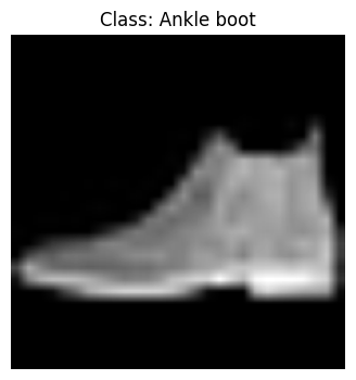

이미지 shape: torch.Size([1, 224, 224])
실제 클래스: Ankle boot (레이블: 9)
예측 클래스: Ankle boot (레이블: 9)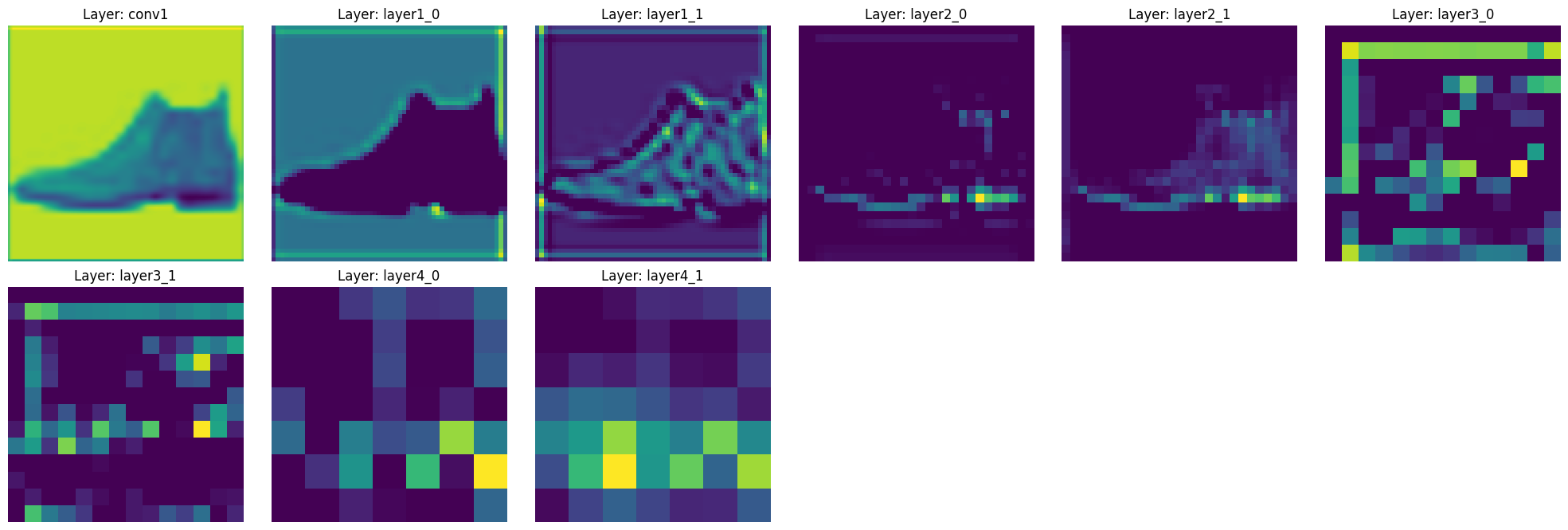

By running this code, you can see how the features change as they pass through the main layers of ResNet-18.

1. Initial convolution (conv1) : Extract basic shape information and low-level features such as edges and textures
2. layer1 (initial residual block) : Combine local features and start simple pattern combinations
3. layer2 : The size of the feature map decreases, but the number of channels increases, recognizing more complex patterns
4. layer3 : With a higher level of abstraction, partial feature detection of objects
5. layer4 (final residual block) : Extract abstract high-level features necessary for class distinction

This hierarchical feature extraction is one of the core strengths of ResNet. Thanks to skip connections, you can see that the features of each layer are well preserved while being gradually abstracted.

Click to view contents (Deep Dive: Inception Module - Adding Diversity and Efficiency to CNN)

Inception Module - Adding Diversity and Efficiency to CNNs

The Inception module is a key component of GoogLeNet, which won the ImageNet Large Scale Visual Recognition Challenge (ILSVRC) in 2014. This module presents a new approach to existing CNN structures, nicknamed “Network in Network”. While ResNet solved the problem of “depth”, the Inception module simultaneously addresses two important issues: “diversity” and “efficiency”. In this deep dive, we will analyze the core ideas, mathematical principles, and evolution of the Inception module, and explore its impact on deep learning, particularly in CNN architecture design.

Core Idea of Inception Module: “Multi-Scale” Feature Extraction

The Inception module provides an elegant solution to this problem by using filters of different sizes in parallel and concatenating their results (feature maps).

Core Ideas:

1. Diverse Filters: Apply convolutional filters of various sizes (e.g., 1x1, 3x3, 5x5) to the same input.
2. Parallel Processing: Each filter performs convolution operations independently.
3. Concatenation: Combine the feature maps generated by each filter along the channel axis.
4. 1x1 Convolution: Reduces computational cost, adds non-linearity, and mixes information between channels (“bottleneck” layer).

Inception Module v1 (GoogLeNet, 2014)

The first version of the Inception module (GoogLeNet) has the following structure:

• Input: Feature map from the previous layer
• Parallel Branches:
  • 1x1 convolution
  • 1x1 convolution -> 3x3 convolution
  • 1x1 convolution -> 5x5 convolution
  • 3x3 max pooling -> 1x1 convolution
• Output: Concatenate the outputs of each branch along the channel axis

Role of 1x1 Convolution:

1x1 convolution plays a crucial role in the Inception module.

• Dimensionality Reduction: 1x1 convolution is used to reduce the number of channels. By using 1x1 convolution before 3x3 or 5x5 convolution, the computational cost can be significantly reduced (bottleneck layer).
• Adding Non-Linearity: Adding an activation function like ReLU after 1x1 convolution introduces non-linearity into the network.
• Mixing Channel Information: 1x1 convolution calculates a linear combination of input channels, effectively mixing information between them.

Limitations of Inception Module v1:

• 5x5 convolution still has a high computational cost.
• Pooling operations can cause information loss while reducing dimensions.

Inception Module v2 & v3 (2015)

Inception v2 and v3 introduced the following ideas to improve upon the limitations of v1:

Version	Improvement
v2	Factorized 5x5 convolution into two 3x3 convolutions
v3	Introduced factorized 7x7 convolution and auxiliary classifiers

These improvements aimed to reduce computational costs while maintaining or improving performance. * Factorization: Decompose a 5x5 convolution into two 3x3 convolutions (reduce computation). * Asymmetric Convolution: Decompose a 3x3 convolution into a 1x3 convolution and a 3x1 convolution. * Auxiliary Classifier: Add an auxiliary classifier during training to mitigate the vanishing gradient problem and accelerate learning (removed in v3). * Label Smoothing: Add a small amount of noise to the correct label to prevent the model from being overconfident.

Inception Module v4 (2016)

Inception-v4 introduced the Inception-ResNet module, combining the Inception module with the residual connection of ResNet [^3].

Xception (2017)

Xception (“Extreme Inception”) is a model that extends the idea of the Inception module to the extreme [^4]. It uses Depthwise Separable Convolution to separate channel-wise spatial convolution (depthwise convolution) and channel-wise convolution (pointwise convolution, 1x1 conv).

Mathematical Expression (Inception v1)

Each branch of the Inception module can be expressed as follows:

• Branch 1: \(\text{Output}_1 = \text{Conv}_{1x1}(\text{Input})\)
• Branch 2: \(\text{Output}_2 = \text{Conv}_{3x3}(\text{Conv}_{1x1}(\text{Input}))\)
• Branch 3: \(\text{Output}_3 = \text{Conv}_{5x5}(\text{Conv}_{1x1}(\text{Input}))\)
• Branch 4: \(\text{Output}_4 = \text{Conv}_{1x1}(\text{MaxPool}(\text{Input}))\)
• Output: \(\text{Concatenate}(\text{Output}_1, \text{Output}_2, \text{Output}_3, \text{Output}_4)\)

Here, \(\text{Conv}_{NxN}\) denotes an \(N \times N\) convolution operation, and \(\text{MaxPool}\) denotes a max pooling operation.

Similarity to Wavelet Transform

The multi-scale approach of the Inception module is similar to the wavelet transform. The wavelet transform is a method for decomposing a signal into various frequency components. Each filter in the Inception module (1x1, 3x3, 5x5) can be interpreted as extracting features at different frequencies or scales. The 1x1 convolution extracts high-frequency components, the 3x3 extracts mid-frequency components, and the 5x5 extracts low-frequency components.

Advantages of Inception Module

• Extracting features at various scales: Using filters of multiple sizes simultaneously effectively captures features of various sizes in an image.
• Computational efficiency: Reducing dimensions using 1x1 convolutions reduces computation while maintaining expressiveness.
• Strong performance: Achieved top-level performance on the ImageNet dataset.

Impact on Deep Learning Ecosystem

The Inception module presented a new perspective on CNN architecture design. It showed that going “deeper” is not the only important thing, but also going “wider” and “more diverse”. The idea of the Inception module later influenced the development of lightweight models such as MobileNet and ShuffleNet.

Simple Inception Module Implementation (PyTorch)

import torch
import torch.nn as nn
import torch.nn.functional as F

class InceptionModule(nn.Module):
    def __init__(self, in_channels, out_channels_1x1, out_channels_3x3_reduce,
                 out_channels_3x3, out_channels_5x5_reduce, out_channels_5x5,
                 out_channels_pool):
        super().__init__()

        # 1x1 conv branch
        self.branch1x1 = nn.Conv2d(in_channels, out_channels_1x1, kernel_size=1)

        # 1x1 conv -> 3x3 conv branch
        self.branch3x3_reduce = nn.Conv2d(in_channels, out_channels_3x3_reduce, kernel_size=1)
        self.branch3x3 = nn.Conv2d(out_channels_3x3_reduce, out_channels_3x3, kernel_size=3, padding=1)

        # 1x1 conv -> 5x5 conv branch
        self.branch5x5_reduce = nn.Conv2d(in_channels, out_channels_5x5_reduce, kernel_size=1)
        self.branch5x5 = nn.Conv2d(out_channels_5x5_reduce, out_channels_5x5, kernel_size=5, padding=2)

        # 3x3 max pool -> 1x1 conv branch
        self.branch_pool = nn.MaxPool2d(kernel_size=3, stride=1, padding=1)
        self.branch_pool_proj = nn.Conv2d(in_channels, out_channels_pool, kernel_size=1)

    def forward(self, x):
        branch1x1 = F.relu(self.branch1x1(x))

        branch3x3 = F.relu(self.branch3x3_reduce(x))
        branch3x3 = F.relu(self.branch3x3(branch3x3))

        branch5x5 = F.relu(self.branch5x5_reduce(x))
        branch5x5 = F.relu(self.branch5x5(branch5x5))

        branch_pool = F.relu(self.branch_pool_proj(self.branch_pool(x)))

        outputs = [branch1x1, branch3x3, branch5x5, branch_pool]
        return torch.cat(outputs, 1)  # Concatenate along the channel dimension

Example Usage

in_channels = 3 # Example input channels out_channels_1x1 = 64 out_channels_3x3_reduce = 96 out_channels_3x3 = 128 out_channels_5x5_reduce = 16 out_channels_5x5 = 32 out_channels_pool = 32

inception_module = InceptionModule(in_channels, out_channels_1x1, out_channels_3x3_reduce, out_channels_3x3, out_channels_5x5_reduce, out_channels_5x5, out_channels_pool)

Example input tensor (batch_size, channels, height, width)

input_tensor = torch.randn(1, in_channels, 28, 28) output_tensor = inception_module(input_tensor) print(output_tensor.shape) # Check output shape

This code implements the basic structure of the Inception Module (v1) using PyTorch. Since more advanced versions of the Inception network (Inception-v3, Inception-v4, Inception-ResNet, etc.) are implemented in libraries such as torchvision.models or timm, it is recommended to use these libraries for actual projects.

---

[1]: Szegedy, C., Liu, W., Jia, Y., Sermanet, P., Reed, S., Anguelov, D., … & Rabinovich, A. (2015). Going deeper with convolutions. In Proceedings of the IEEE conference on computer vision and pattern recognition (pp. 1-9).

[2]: Szegedy, C., Vanhoucke, V., Ioffe, S., Shlens, J., & Wojna, Z. (2016). Rethinking the inception architecture for computer vision. In Proceedings of the IEEE conference on computer vision and pattern recognition (pp. 2818-2826).

[3]: Szegedy, C., Ioffe, S., Vanhoucke, V., & Alemi, A. A. (2017). Inception-v4, inception-resnet and the impact of residual connections on learning. In Thirty-first AAAI conference on artificial intelligence.

[4]: Chollet, F. (2017). Xception: Deep learning with depthwise separable convolutions. In Proceedings of the IEEE conference on computer vision and pattern recognition (pp. 1251-1258).

7.3 EfficientNet: Efficient Model Scaling

Challenge: How can we maximize the performance of a model while minimizing its computational cost (number of parameters, FLOPS)?

Researcher’s Dilemma: With the advent of ResNet, it became possible to train deep networks, but there was no systematic way to adjust the size of the model. Simply adding more layers or increasing the number of channels could greatly increase the computational cost. Researchers sought to find the optimal balance between the depth, width, and resolution of a model to achieve the best performance under given computational resources.

7.3.1 Compound Scaling: Balancing Depth, Width, and Resolution

The core idea of EfficientNet is “Compound Scaling.” While previous studies tended to adjust only one of the depth, width, or resolution, EfficientNet found that adjusting all three factors simultaneously and in a balanced way is more efficient.

• Depth: The number of layers in the network. Deeper networks can learn more complex features but are prone to vanishing/exploding gradient problems and overfitting.
• Width: The number of channels (filters) in each layer. Wider networks can learn finer-grained features but increase computational cost and parameter count, risking overfitting.
• Resolution: The size of the input image. Higher resolution images contain more information but greatly increase computational cost.

EfficientNet experimentally showed that these three factors are interrelated and that adjusting them together in a balanced way is more effective than changing one factor alone. For example, if the image resolution is doubled, the network should be deepened and widened appropriately to learn finer patterns; simply increasing the resolution may result in minimal or even decreased performance.

The EfficientNet paper defines the model scaling problem as an optimization problem and expresses the relationship between depth, width, and resolution using the following formula.

First, let’s denote a CNN model as \(\mathcal{N}\). The \(i\)th layer can be represented as a function transformation \(Y_i = \mathcal{F}_i(X_i)\), where \(Y_i\) is the output tensor, \(X_i\) is the input tensor, and \(\mathcal{F}_i\) is the operator. The shape of the input tensor \(X_i\) can be expressed as \(<H_i, W_i, C_i>\), which represents height, width, and channel count, respectively.

The entire CNN model \(\mathcal{N}\) can be represented as the composition of each layer’s function:

\(\mathcal{N} = \mathcal{F}_k \circ \mathcal{F}_{k-1} \circ ... \circ \mathcal{F}_1 = \bigodot_{i=1...k} \mathcal{F}_i\)

While typical CNN designs focus on finding the optimal layer operation \(\mathcal{F}_i\), EfficientNet focuses on adjusting the length (\(\hat{L}_i\)), width (\(\hat{C}_i\)), and resolution (\(\hat{H}_i, \hat{W}_i\)) of the network, with the layer operations fixed. To do this, a baseline network is defined as \(\hat{\mathcal{N}}\), and the model is expanded by multiplying scaling coefficients. Benchmark network: \(\hat{\mathcal{N}} = \bigodot_{i=1...s} \hat{\mathcal{F}}_i^{L_i}(X_{<H_i, W_i, C_i>})\)

EfficientNet aims to solve the following optimization problem:

\(\underset{\mathcal{N}}{maximize}\quad Accuracy(\mathcal{N})\)

\(subject\ to\quad \mathcal{N} = \bigodot_{i=1...s} \hat{\mathcal{F}}_i^{d \cdot \hat{L}_i}(X_{<r \cdot \hat{H}_i, r \cdot \hat{W}_i, w \cdot \hat{C}_i>})\)

\(Memory(\mathcal{N}) \leq target\_memory\)

\(FLOPS(\mathcal{N}) \leq target\_flops\)

Here, \(d\), \(w\), \(r\) are the scaling coefficients for depth, width, and resolution, respectively.

To solve this problem, EfficientNet proposes a Compound Scaling method that simplifies the complex optimization problem by maximizing accuracy while satisfying all resource constraints. Compound scaling adjusts depth, width, and resolution uniformly using a single coefficient (\(\phi\), compound coefficient).

\(\begin{aligned} & \text{depth: } d = \alpha^{\phi} \\ & \text{width: } w = \beta^{\phi} \\ & \text{resolution: } r = \gamma^{\phi} \\ & \text{subject to } \alpha \cdot \beta^2 \cdot \gamma^2 \approx 2 \\ & \alpha \geq 1, \beta \geq 1, \gamma \geq 1 \end{aligned}\)

• \(\phi\) (phi) is a user-specified coefficient that controls the overall model size.
• \(\alpha\), \(\beta\), \(\gamma\) are constants that determine how much to increase the depth, width, and resolution, respectively. These values are determined through a small grid search. (To find the values of \(\alpha\), \(\beta\), \(\gamma\), we fix \(\phi=1\) and perform a small search.)
• The constraint (\(\alpha \cdot \beta^2 \cdot \gamma^2 \approx 2\)) is set so that when \(\phi\) increases by 1, the model’s FLOPS approximately doubles. This constraint is set because FLOPS increase linearly with depth and quadratically with width and resolution.

Using this compound scaling method, users can easily adjust the model size by tuning a single value (\(\phi\)) and effectively control the balance between model performance and efficiency.

7.3.2 EfficientNet Architecture

EfficientNet uses AutoML (Neural Architecture Search, NAS) technology to find the optimal baseline model, EfficientNet-B0, and applies compound scaling to create models of various sizes (B1 ~ B7, and larger L2).

Structure of EfficientNet-B0:

EfficientNet-B0 is based on the MBConv (Mobile Inverted Bottleneck Convolution) block, which is inspired by MobileNetV2. The MBConv block has the following structure to increase computational efficiency:

Layer	Output Size	Number of Layers	Number of Parameters
Stem	32x32x16	1	-
MBConv1	32x32x16	1	-
MBConv2	16x16x24	2	-
MBConv3	8x8x40	2	-
MBConv4	4x4x80	3	-
MBConv5	2x2x112	3	-
MBConv6	1x1x192	4	-
Head	1x1x1280	1	-

Note: The number of layers and parameters in each block are not specified in the original text, so this table is incomplete.

EfficientNet-B0 uses a combination of MBConv blocks with different output sizes and numbers of layers to achieve efficient computation. 1. Expansion (1x1 Conv): Expands the number of input channels (expansion factor, usually 6). By increasing the channel count using 1x1 convolution, it can relatively reduce the computational cost of subsequent operations (depthwise convolution) while increasing expressiveness.

2. Depthwise Separable Convolution:

   • Depthwise Convolution (3x3): Performs spatial convolution independently for each input channel. Unlike regular convolution, there is no mixing of information between channels.
   • Pointwise Convolution (1x1 Conv): Uses 1x1 convolution to mix information between channels.

   Depthwise separable convolution can greatly reduce the number of parameters and computations compared to regular convolution.

3. Squeeze-and-Excitation (SE) Block: Learns the importance of each channel and emphasizes important ones. The SE block uses global average pooling to summarize the information of each channel and two fully connected layers to calculate channel-wise weights.

4. Projection (1x1 Conv): Reduces the number of channels back to the original count (for residual connection).

5. Residual Connection: Adds the input and output together (when the input and output channel counts are the same, with stride=1). This is a core idea of ResNet.

The following is an example implementation of the MBConv block of EfficientNet-B0 using PyTorch. (The full implementation of EfficientNet-B0 is omitted and can be imported from torchvision or timm libraries.)

import torch
import torch.nn as nn
import torch.nn.functional as F

class MBConvBlock(nn.Module):
    def __init__(self, in_channels, out_channels, stride, expand_ratio=6, se_ratio=0.25, kernel_size=3):
        super().__init__()

        self.stride = stride
        self.use_residual = (in_channels == out_channels) and (stride == 1) # 잔차 연결 조건

        expanded_channels = in_channels * expand_ratio

        # Expansion (1x1 conv)
        self.expand_conv = nn.Conv2d(in_channels, expanded_channels, kernel_size=1, bias=False)
        self.bn0 = nn.BatchNorm2d(expanded_channels)

        # Depthwise convolution
        self.depthwise_conv = nn.Conv2d(expanded_channels, expanded_channels, kernel_size=kernel_size,
                                       stride=stride, padding=kernel_size//2, groups=expanded_channels, bias=False)
                                       # groups=expanded_channels: depthwise conv
        self.bn1 = nn.BatchNorm2d(expanded_channels)

        # Squeeze-and-Excitation
        num_reduced_channels = max(1, int(in_channels * se_ratio))  # 최소 1개는 유지
        self.se_reduce = nn.Conv2d(expanded_channels, num_reduced_channels, kernel_size=1)
        self.se_expand = nn.Conv2d(num_reduced_channels, expanded_channels, kernel_size=1)

        # Pointwise convolution (projection)
        self.project_conv = nn.Conv2d(expanded_channels, out_channels, kernel_size=1, bias=False)
        self.bn2 = nn.BatchNorm2d(out_channels)

    def forward(self, x):
        identity = x

        # Expansion
        out = F.relu6(self.bn0(self.expand_conv(x)))

        # Depthwise separable convolution
        out = F.relu6(self.bn1(self.depthwise_conv(out)))

        # Squeeze-and-Excitation
        se = out.mean((2, 3), keepdim=True)  # Global Average Pooling
        se = F.relu6(self.se_reduce(se))
        se = torch.sigmoid(self.se_expand(se))
        out = out * se  # 채널별 가중치 곱

        # Projection
        out = self.bn2(self.project_conv(out))

        # Residual connection
        if self.use_residual:
            out = out + identity

        return out

# Example usage
# in_channels = 32
# out_channels = 16
# stride = 1
# mbconv_block = MBConvBlock(in_channels, out_channels, stride)
# input_tensor = torch.randn(1, in_channels, 224, 224)  # Example input
# output_tensor = mbconv_block(input_tensor)
# print(output_tensor.shape)

7.3.3 EfficientNet’s Performance and Impact

EfficientNet achieved higher accuracy with much fewer parameters and computations than existing CNN models (ResNet, DenseNet, Inception, etc.) on ImageNet classification. The table below compares the performance of EfficientNet and other models.

Model	Top-1 Accuracy	Top-5 Accuracy	Parameters	FLOPS
ResNet-50	76.0%	93.0%	25.6M	4.1B
DenseNet-169	76.2%	93.2%	14.3M	3.4B
Inception-v3	77.9%	93.8%	23.9M	5.7B
EfficientNet-B0	77.1%	93.3%	5.3M	0.39B
EfficientNet-B1	79.1%	94.4%	7.8M	0.70B
EfficientNet-B4	82.9%	96.4%	19.3M	4.2B
EfficientNet-B7	84.3%	97.0%	66M	37B
EfficientNet-L2*	85.5%	97.7%	480M	470B

• Noisy Student Training used

As shown in the table, EfficientNet-B0 achieved higher accuracy with fewer parameters and FLOPS than ResNet-50. EfficientNet-B7 achieved a state-of-the-art 84.3% Top-1 accuracy on ImageNet at the time, while still being much more efficient than other large models.

EfficientNet’s Key Contributions:

• Compound Scaling: A new methodology that balances model depth, width, and resolution, increasing understanding of the relationship between model size and performance.
• Efficient Model Design: EfficientNet-B0, found using AutoML (NAS), showed more efficient and powerful performance than manually designed models.
• Practicality: EfficientNet provides various sizes of models (B0 ~ B7, L2) for users to choose according to their computing resources and performance requirements.

Impact on Academia and Industry:

EfficientNet has promoted research in model lightweighting and efficiency and is widely used in deploying deep learning models in resource-constrained environments such as mobile devices and embedded systems. The compound scaling idea of EfficientNet has been applied to other models, resulting in improved performance. After EfficientNet, follow-up studies emphasizing efficiency, such as EfficientNetV2, MobileNetV3, and RegNet, have been actively conducted.

Limitations:

• There is still a lack of complete theoretical explanation for why the EfficientNet-B0 architecture found using AutoML (NAS) is more effective than other architectures.
• The compound scaling method cannot guarantee optimality for all types of CNN architectures and tasks. Despite this, EfficientNet is considered a significant milestone in the history of deep learning, as it presents a new perspective on CNN model design and greatly improves the efficiency of the model.

Conclusion

In this chapter, we explored the background and development process of convolutional neural networks (CNNs), and examined the most important developments in CNNs, including ResNet, Inception modules, and EfficientNet.

CNNs have achieved great success in image recognition, from early models like LeNet-5 and AlexNet, but faced difficulties in learning deep networks. ResNet solved this problem using residual connections, enabling a significant increase in depth. The Inception module improved the diversity and efficiency of feature extraction by using filters of various sizes in parallel, while EfficientNet presented a systematic method for balancing model depth, width, and resolution.

These innovations have greatly contributed to CNNs playing a core role in various computer vision tasks beyond image recognition. However, CNNs are strong in capturing spatial local patterns but are not suitable for sequential data, especially natural language processing, where order and long-range dependencies are important.

In the next chapter, we will explore the Transformer architecture, which models relationships between elements in a sequence using only the Attention mechanism, without convolutional or pooling operations. The Transformer has brought about significant performance improvements in natural language processing and is now expanding its influence to various fields such as computer vision and speech processing. Just as ResNet’s residual connections overcame the depth limitations of CNNs, the Transformer’s Attention mechanism has opened up new horizons for sequence data processing.

Practice Problems

Basic Problems

1. Explain the role of convolution operations in image processing and provide a specific example using the Sobel filter.
2. Describe the role and advantages of pooling layers in CNNs and compare the differences between max pooling and average pooling.
3. Explain how residual connections, the core idea of ResNet, help with deep network learning, relating it to the vanishing/exploding gradient problem.
4. Describe the core ideas of Inception modules, including “using filters of various sizes” and “1x1 convolution,” and their roles.
5. Explain what EfficientNet’s “compound scaling” is and compare its advantages to traditional model size adjustment methods (adjusting depth, width, or resolution).

Applied Problems

1. Implement a simple CNN model using PyTorch, train and evaluate it using the MNIST dataset (including data loading, model definition, training loop, and evaluation loop).
2. Load the ResNet-18 model from torchvision.models and perform transfer learning on the CIFAR-10 dataset, evaluating its performance (including data preprocessing, model loading, fine-tuning, and evaluation).
3. Use the provided show_filter_effects function in expertai_src to visually compare the effects of various filters (blur, sharpen, edge detection, etc.) on images and describe each filter’s characteristics.
4. Remove residual connections from the given ResNet code (BasicBlock, Bottleneck) and measure the change in performance when trained on the same data, analyzing the reasons for this change.
5. Implement 2D convolution operations directly using the SimpleConv2d class as a reference (using NumPy or PyTorch’s tensor operations, without using torch.nn.Conv2d).

Advanced Problems

1. Mathematically explain why vanishing/exploding gradient problems occur in deep CNNs and describe how ResNet’s residual connections, batch normalization, and Inception modules’ 1x1 convolutions alleviate these issues.
2. Read the ResNet, Inception, and EfficientNet papers and compare their core ideas, analyzing each model’s advantages and disadvantages, relationships between them, and their impact on subsequent research.
3. Derive (or explain in detail using the paper) EfficientNet’s compound scaling formula and describe how to determine the optimal model size under given computational resource constraints.
4. Explain the relationship between Gaussian processes and deep kernel learning (DKL), describing DKL’s advantages over traditional CNNs and GPs.
5. Find examples of recent (within the last 1-2 years) CNN-related papers that build upon ResNet, Inception, and EfficientNet ideas, summarize their content, and provide your own perspective (e.g., ConvNeXt, NFNet).

Click to view contents (exercise answers)

Exercise Answers

Basic Problems

1. Role of Convolution and Sobel Filter:
   • Role: Convolution extracts features by operating on an image and a filter (kernel), calculating the weighted sum of pixel values and filter values as the filter moves over the image.
   • Sobel Filter: Used for edge detection in images. Vertical/horizontal Sobel filters detect brightness changes in vertical/horizontal directions.
2. Pooling Layer:
   • Role/Advantage: Reduces the size (spatial dimension) of feature maps, decreasing computation and increasing translational invariance to prevent overfitting.
   • Max Pooling: Selects the maximum value in a region, preserving the most prominent features.
   • Average Pooling: Calculates the average value in a region, being less sensitive to noise.
3. ResNet Residual Connection:
   • Residual Connection: A “shortcut” connection that directly adds input values to output values. \(H(x) = F(x) + x\)
   • Gradient Vanishing/Exploding Mitigation: Gradients are directly propagated through residual connections, allowing them to flow well even in deep networks. Helps the neural network learn the identity mapping (\(F(x) = 0\)) easily.
4. Inception Module:
   • Filters of Various Sizes: Uses filters of different sizes (1x1, 3x3, 5x5, etc.) in parallel to capture features of various sizes in an image simultaneously.
   • 1x1 Convolution: Reduces dimensionality between channels and adds non-linearity. Increases model expressiveness while reducing computation (“bottleneck” layer role).
5. EfficientNet Compound Scaling:
   • Compound Scaling: A method that increases the depth, width, and resolution of a network in a balanced way, using a single compound coefficient to adjust all three factors.
   • Advantage: More efficiently improves model performance than existing methods (which change one factor at a time). Allows for optimal performance under given computational resource constraints by adjusting model size.

Application Problems

1. CNN Implementation and MNIST Training: (Code omitted) Implements a CNN model using PyTorch’s nn.Conv2d, nn.ReLU, nn.MaxPool2d, nn.Linear, etc., and trains it on the MNIST dataset using DataLoader.

2. ResNet-18 Transfer Learning: (Code omitted) Loads resnet18 from torchvision.models, replaces the last layer (fully connected layer) to fit CIFAR-100, and fine-tunes some layers.

3. Analysis of show_filter_effects: (Code omitted) The show_filter_effects function applies various filters (Gaussian Blur, Sharpen, Edge Detection, Emboss, Sobel X) to a given image and visualizes the results. Each filter emphasizes or transforms specific image features (blurriness, sharpness, edge detection, etc.).

4. Removing ResNet Residual Connections: (Code omitted) Removing residual connections tends to make deep network training more difficult due to gradient vanishing/exploding problems, leading to decreased performance.

5. 2D Convolution Direct Implementation: (code omitted) Uses nested for loops to perform element-wise multiplication and summation between the input tensor and the kernel at each position. It is more efficient to convert it into matrix multiplication using techniques such as im2col.

Advanced Problems

1. Vanishing/Exploding Gradient:

   • Cause: During backpropagation, gradients are repeatedly multiplied according to the chain rule, resulting in very small (vanishing) or large (exploding) gradients as you go deeper. If the derivative of the activation function is less than 1 (e.g., sigmoid, tanh), it tends to vanish, and if it’s greater than 1, it tends to explode.
   • ResNet Residual Connection: Gradients are directly passed through residual connections, alleviating the vanishing/exploding gradient problem.
   • Batch Normalization: Normalizes the input of each layer to keep the activation function’s input within an appropriate range, reducing vanishing/exploding gradients.
   • Inception 1x1 Convolution: Reduces the number of channels, decreasing computation and indirectly alleviating vanishing/exploding gradients (due to fewer parameters).

2. ResNet, Inception, EfficientNet Comparison: (detailed comparison omitted)

   • ResNet: Enables deep network learning through residual connections.
   • Inception: Uses parallel filters of various sizes to extract features at different scales and improves computational efficiency with 1x1 convolutions.
   • EfficientNet: Improves both efficiency and performance by balancing model depth, width, and resolution using Compound Scaling.

3. EfficientNet Compound Scaling: (formula derivation/detailed explanation omitted) Uses a compound coefficient (Φ) to adjust depth (α^Φ), width (β^Φ), and resolution (γ^Φ). α, β, and γ are constants found through small grid searches. Constraint: α ⋅ β² ⋅ γ² ≈ 2.

4. Gaussian Process (GP) and DKL:

   • GP: A probability distribution over functions. Defines covariance between function values using a kernel function. Provides prediction uncertainty through Bayesian inference.
   • DKL (Deep Kernel Learning): Uses deep learning (neural networks) to extract features from data and uses these features as inputs to the GP’s kernel function. Combines deep learning’s representation learning capability with GP’s uncertainty estimation ability.
   • Advantages: Data efficiency, uncertainty estimation, flexible feature representation.
   • Disadvantages: GP’s computational complexity still exists.

5. Latest CNN Papers: (e.g., ConvNeXt, NFNet, etc.; paper summaries and opinions omitted)

References

1. Receptive fields, binocular interaction and functional architecture in the cat’s visual cortex (Hubel & Wiesel, 1962): A study on the cat’s visual cortex that inspired the concept of receptive fields in CNNs. (https://www.ncbi.nlm.nih.gov/pmc/articles/PMC1359523/)
2. The Scientist and Engineer’s Guide to Digital Signal Processing (Steven W. Smith): A book that explains the basic principles of digital signal processing, helping to understand convolution, filters, etc. (http://www.dspguide.com/pdfbook.htm)
3. Gradient-based learning applied to document recognition (LeCun et al., 1998): A paper on character recognition using CNNs, introducing LeNet-5. (http://vision.stanford.edu/cs598_spring07/papers/Lecun98.pdf)
4. Deep Residual Learning for Image Recognition (He et al., 2015): The original paper on ResNet. (https://arxiv.org/pdf/1512.03385.pdf)
5. Network in Network (Lin et al., 2013): A paper that proposed the idea of 1x1 convolution. (https://arxiv.org/pdf/1312.4400.pdf)
6. Very Deep Convolutional Networks for Large-Scale Image Recognition (Simonyan & Zisserman, 2014): The paper on VGGNet. (https://arxiv.org/pdf/1409.1557.pdf)
7. Dive into Deep Learning (Zhang et al., 2023): Chapter 9 “Convolutional Neural Networks” explains the basic concepts of CNNs and ResNet. (https://d2l.ai/chapter_convolutional-neural-networks/index.html)
8. CS231n: Convolutional Neural Networks for Visual Recognition (Stanford University): Lecture materials on CNNs. (http://cs231n.github.io/convolutional-networks/)
9. Understanding the Disharmony between Dropout and Batch Normalization by Variance Shift (Li et al., 2018): A paper that explains the precautions to take when using batch normalization and dropout together.
10. Rethinking the Inception Architecture for Computer Vision (Szegedy et al., 2015): Explains Inception-v3 and the inception module. (https://arxiv.org/abs/1512.00567)
11. Receptive fields, binocular interaction and functional architecture in the cat’s visual cortex (Hubel & Wiesel, 1962): A study on the cat’s visual cortex that inspired the concept of receptive fields in CNNs. (https://www.ncbi.nlm.nih.gov/pmc/articles/PMC1359523/) 2. The Scientist and Engineer’s Guide to Digital Signal Processing (Steven W. Smith): A book that explains the basic principles of digital signal processing, helping to understand convolution, filters, etc. (http://www.dspguide.com/pdfbook.htm) 3. Gradient-based learning applied to document recognition (LeCun et al., 1998): A paper on character recognition using CNNs, introducing LeNet-5. (http://vision.stanford.edu/cs598_spring07/papers/Lecun98.pdf) 4. Deep Residual Learning for Image Recognition (He et al., 2015): The original paper on ResNet. (https://arxiv.org/pdf/1512.03385.pdf) 5. Network in Network (Lin et al., 2013): A paper that proposed the idea of 1x1 convolution. (https://arxiv.org/pdf/1312.4400.pdf) 6. Very Deep Convolutional Networks for Large-Scale Image Recognition (Simonyan & Zisserman, 2014): The paper on VGGNet. (https://arxiv.org/pdf/1409.1557.pdf) 7. Dive into Deep Learning (Zhang et al., 2023): Chapter 9 “Convolutional Neural Networks” explains the basic concepts of CNNs and ResNet. (https://d2l.ai/chapter_convolutional-neural-networks/index.html) 8. CS231n: Convolutional Neural Networks for Visual Recognition (Stanford University): Lecture materials on CNNs. (http://cs231n.github.io/convolutional-networks/) 9. Understanding the Disharmony between Dropout and Batch Normalization by Variance Shift (Li et al., 2018): A paper that explains the precautions to take when using batch normalization and dropout together. 10. Rethinking the Inception Architecture for Computer Vision (Szegedy et al., 2015): A paper that explains Inception-v3 and the inception module. There is no text to translate. The provided text only contains instructions and a link, but does not include any Korean text that needs to be translated into English.